![]()
![]()
| Related Topics: | ||
![]()
An analyst is performing a field test for a prototype product. A group of 21 participants agreed to test the product and all participants are to return after appointed periods of time to report their experience with the product.
Units that are reported to have malfunctioned during the test period are marked as failed (F), while units that did not exhibit any problems are marked as suspensions (S). At the end of the 35 week test, the analyst’s log shows the following information.
| Number of Units | State (F or S) | Test Period (Weeks) |
| 3 | F | 9 |
| 1 | S | 9 |
| 1 | F | 11 |
| 1 | S | 12 |
| 1 | F | 13 |
| 1 | S | 13 |
| 1 | S | 15 |
| 1 | F | 17 |
| 1 | F | 21 |
| 1 | S | 22 |
| 1 | S | 24 |
| 1 | S | 26 |
| 1 | F | 28 |
| 1 | F | 30 |
| 5 | S | 35 |
The objective is to create a Reliability vs. Time plot in order to predict the failure rate behavior of the product.
The first step is to create a non-parametric LDA folio. Choose Insert > Folios > Non-Parametric LDA.
![]()
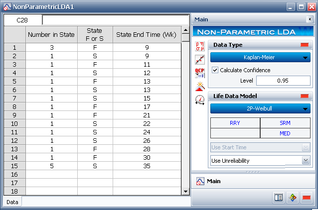
On the Main page of the control panel, choose the Kaplan-Meier analysis. This will format the data sheet correctly for the non-parametric analysis. Select the Calculate Confidence check box and enter 0.95 for the confidence level.
Click the Change Units icon.
![]()
In the Change Units window, change the time unit to Week. Click OK.
Next, enter the information from the table in the data sheet.
The non-parametric LDA folio will obtain the reliability estimates only for the failure times that were entered in the data sheet (in this example, it is for weeks 9, 11, 13, 17, 21, 28 and 30). In order to estimate (i.e., interpolate) the reliability of the product at other times, you will need to create a parametric model. To do this, make the following selections in the Life Data Model area of the control panel:
2P-Weibull.
RRY (Rank Regression on Y).
Use Unreliability. This means that the free-form data set will be based on the unreliability estimates calculated from the non-parametric analysis, rather than the upper or lower confidence bound.
The following picture shows the completed setup.
Choose Non-Parametric LDA > Analysis > Calculate or click the icon on the control panel.
![]()
The software will perform a non-parametric analysis on the data set, and then automatically perform a separate standard life data analysis based on the settings specified in the Life Data Model area.
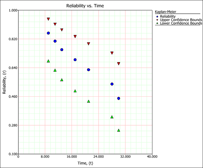
To create the Reliability vs. Time plot, choose Non-Parametric LDA > Analysis > Plot or click the icon on the control panel.
![]()
In the following example, the dots on the plot show the reliability estimates at each point of failure, the triangles show the lower 1-sided confidence bounds of the estimates, and the inverted triangles show the upper 1-sided confidence bounds. The pattern of the data points shows that the product exhibits a sharp decline in reliability over the course of a few weeks.
To view the calculated reliability values, click the Non-Parametric Results (...) button on the control panel to open the Results window, as shown next.
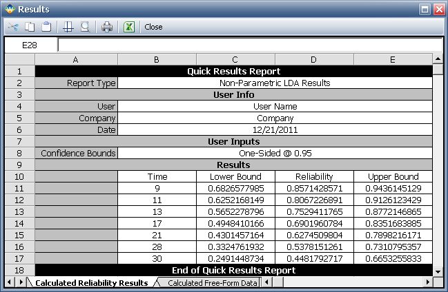
The results show that the reliability of the product at 9 weeks of operation is estimated to be 85.71%; however, by 30 weeks, the reliability estimate is 44.81% and may be as low as 24.91%.
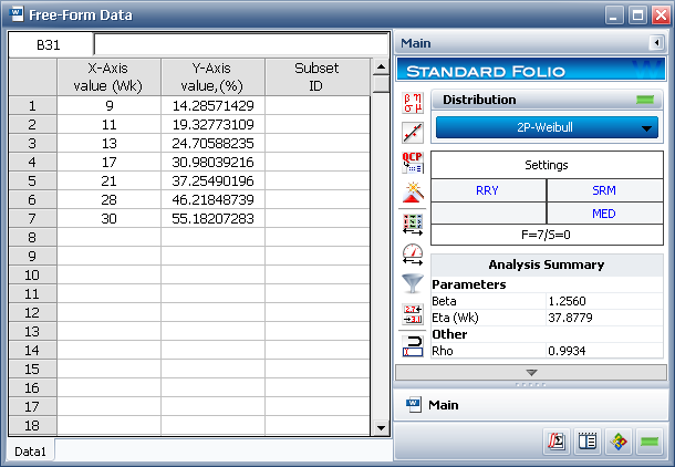
To assess whether the assumed distribution (that was chosen in the Life Data Model area of the control panel) provides a good fit, you can transfer the results of the non-parametric analysis to a Weibull++ standard folio. To do this, choose Non-Parametric LDA > Transfer Life Data > Transfer Life Data to a New Folio.
![]()
The data will be transferred to a free-form data sheet, where the failure time values will be copied to the “X-Axis value” column, and the unreliability values will be copied to the “Y-Axis value” column.
In the standard folio, select the same analysis settings that you chose in the non-parametric LDA folio (i.e., 2P-Weibull and RRY), and then click the Calculate icon on the control panel. The following picture shows the completed analysis.
Next, click the Plot icon on the control panel. The following probability plot shows the probability line with respect to the values obtained from the non-parametric analysis. As you can see, the 2P-Weibull provides a good fit to the values.
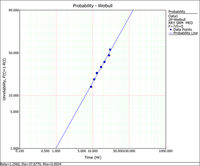
If the distribution did not provide a good fit, you could experiment with other distributions to see which one would provide a better fit. Once you have selected an appropriate parametric model, you can use it to obtain calculations from the Quick Calculation Pad (QCP).
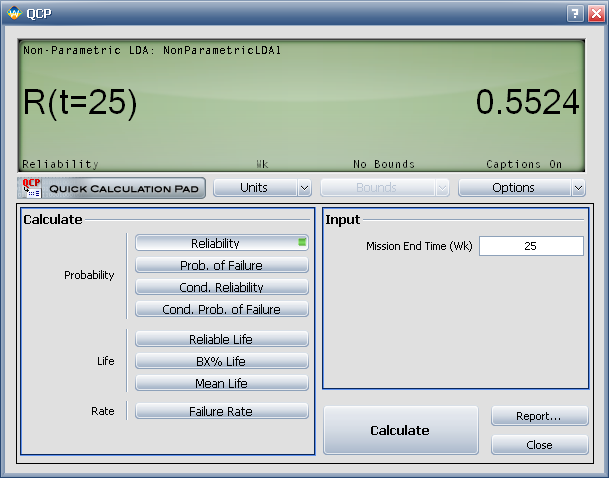
To obtain a reliability estimate at a time that was not calculated in the non-parametric analysis, say, 25 weeks, use the Quick Calculation Pad (QCP). You can use the QCP either from the standard folio with the transferred data or from the non-parametric LDA folio. If you use the same analysis settings (i.e., distribution, parameter estimation method) in both the standard folio and non-parametric LDA folio, then you will obtain the same results from the QCPs in both folios.
Click the QCP icon on the control panel.
![]()
In the QCP, choose to calculate the Reliability. Select Week for the time units and then enter 25 for the mission end time. Click Calculate to display the results. The reliability is 55.24%, as shown next.
Note: Confidence bounds calculations are not available for free-form data.
© 1992-2013. ReliaSoft Corporation. ALL RIGHTS RESERVED.