![]()
![]()
The data set used in this example is available in the example database installed with the software (called "DOE11_examples.rsgz11"). To access this database file, choose File > Help, click Open Examples Folder, then browse for the file in the DOE sub-folder.
The name of the example project is "Reliability DOE - Optimization for a Single Response."
In this example, two factors in a manufacturing process, curing temperature and curing time, have a significant effect on the life of a component. A central composite design is used to investigate the relationship between these factors and the life of the component. Life is defined as cycles-to-failure under normal use conditions. The warranty period is 1,000 cycles.
5 units are available for testing, and the factors and levels shown next will be used.
|
Factor |
Low Level |
High Level |
|
Temperature (degrees C) |
80 |
100 |
|
Time (min) |
300 |
500 |
A reasonable reliability should be achieved for the warranty period. If the reliability is too low, the warranty cost will be high. If the product is overdesigned or too reliable, then customers will not replace their old components, which will negatively affect sales. The target reliability is decided to be 0.95 and values below 0.92 or above 0.98 are considered unacceptable. The goal of the experiment is to find the optimal settings of temperature and time.
The design matrix and the response data are given in the "Central Composite R-DOE" folio. The following steps describe how to create this folio on your own.
Choose Insert > Designs > Standard Design to add a standard design folio to the current project.
Click Design Type in the folio's navigation panel, and then select Central Composite Response Surface Method in the input panel.
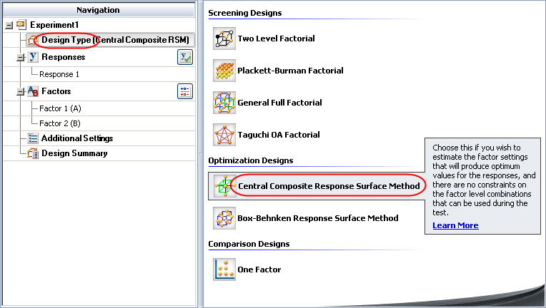
Rename the folio by clicking the Experiment1 heading in the navigation panel and entering Central Composite R-DOE for the Name in the input panel.
Specify that you will be performing reliability DOE by clicking Response 1 in the navigation panel and choosing Life Data from the Response Type drop-down list. Then choose Suspensions from the Censoring drop-down list to specify that some of the data points will be suspensions (i.e., times at which the unit was found not failed). Rename the response to Cycle to Failure.
Define each factor by clicking it in the navigation panel and editing its properties in the input panel. The first factor is shown next.
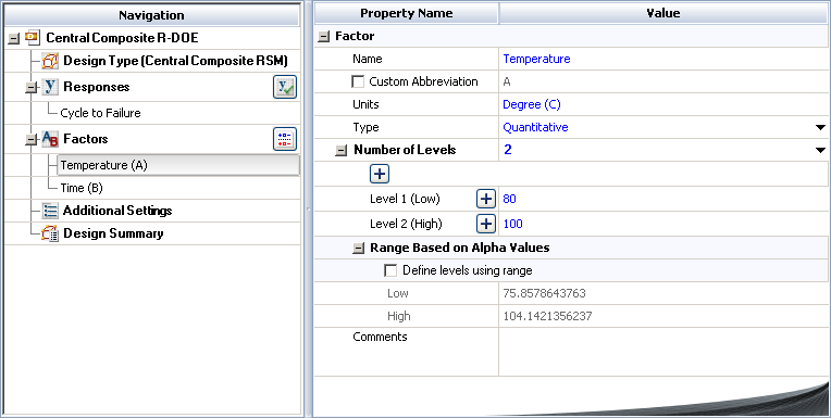
See Adding, Removing and Editing Factors.
Click the Additional Settings heading to choose the number of replicates, specify the kind of fractional design that will be used and define the generators (i.e., aliased effects).
Set the number of Replicates to 5 (since there are 5 units tested for each factor level combination).
Choose Yes from the Block on Replicates drop-down list. This specifies that each replicate will be assigned its own block in the design.
Finally, click the Build icon on the control panel to create a Data tab that allows you to view the test plan and enter response data.
![]()
The data set for this example is given in the "Central Composite R-DOE" folio of the example project. After you enter the data from the folio, you can perform the analysis by doing the following:
Note: To minimize the effect of unknown nuisance factors, the run order is randomly generated when you create the design. Therefore, if you followed these steps to create your own folio, the order of runs on the Data tab may be different from that of the folio in the example file. This can lead to different results. To ensure that you get the very same results described next, show the Standard Order column in your folio, then click a cell in that column and choose Sheet > Sheet Actions > Sort > Sort Ascending. This will make the order of runs in your folio the same as that of the example file. Then copy the response data from the example file and paste it into the Data tab of your folio.
On the Analysis Settings page of the control panel, select to use Individual Terms in the analysis.
Return to the Main page of the control panel and click the Calculate icon.
![]()
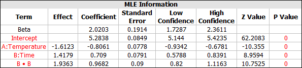
Click the View Analysis Summary icon on the control panel and select to the view the MLE Information table.
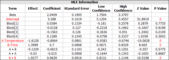
From this table, you can see that effects A and B, as well as the quadratic effect of B (i.e., B·B), are significant. To simply the analysis, the next step is to recreate the model using only the significant terms.
The results for the reduced model are given in the "Reduced Model" folio of the example project. The following steps describe how to create this folio on your own in order to generate the regression model that will be used for the optimization.
Right-click the design folio in the current project explorer and select Duplicate Item from the shortcut menu. Rename the new folio with an appropriate name.
Click the Select Terms icon on the new folio's control panel.
![]()
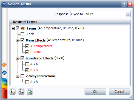
In the Select Terms window that appears, click the Select Significant Effects button to select only the significant effects to calculate the new model, as shown next, then click OK.
Click the Calculate icon in the new folio's control panel.
To see the details of the reduced model, view the MLE Information table.
The optimal factor settings are available in the "Optimization" folio of the example project. Follow the steps outlined below to create the folio from scratch and solve for the optimal settings.
On the control panel of the "Reduced Model" standard design folio, click the Optimization icon.
![]()
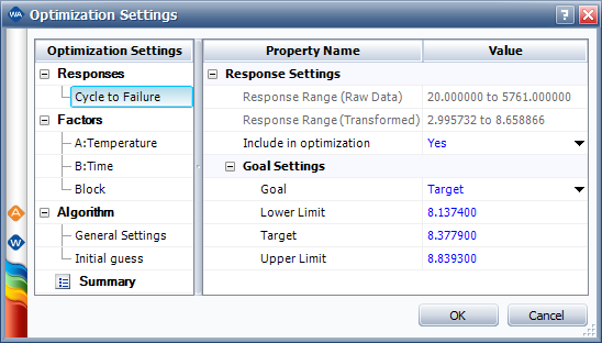
The Optimization Settings window will appear. Click the cell in the Goal column and choose Target from the drop-down list. Then, enter the target response value, as well as the lower and upper limits on the value.
When you enter target values to optimize a life data response, the values must be entered in terms of ln(eta) for the Weibull distribution. From the MLE Information table, we know that beta = 2.0203. If you assume that beta is the same under different factor values and that only the scale parameter is affected by the factor values, then you can use the required reliability value to calculate the required eta.
The reliability function for a Weibull distribution is:
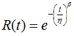
Therefore, since the target reliability is 0.95, the target eta is 4,350. Similarly, the lower (0.92) and upper (0.98) limits on the reliability are equivalent to eta values of 3,420 and 6,900, respectively.
In the software, we assume the logarithmic transform of eta is a linear function of all the effects. For this example, it is:
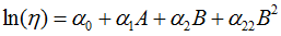
So the logarithmic transform is used in the optimization. In this case the lower limit is 8.1374, the target value is 8.3779 and the upper limit is 8.8393. After entering the values, the window will appear as shown next.
Click OK to calculate the optimal solutions. The first solution will be shown in the plot. To view all the numerical solutions at once, click the View Solutions icon ( ![]() ) at the bottom of the control panel. Four optimal solutions will be shown.
) at the bottom of the control panel. Four optimal solutions will be shown.
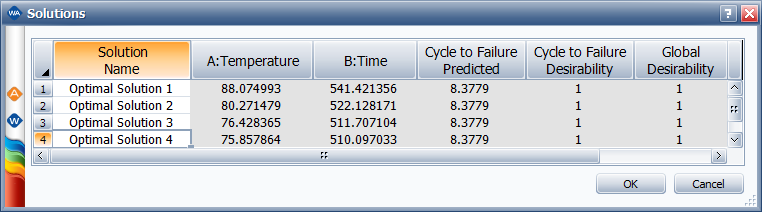
In this example, optimal solution 4 uses the shortest curing time and lowest temperature among all the 4 solutions. Therefore, it can be used as the final recommended factor setting.
© 1992-2017. HBM Prenscia Inc. ALL RIGHTS RESERVED.
 |
E-mail Link |