	Related Topics:
	Spreadsheets

Spreadsheet Example

The data set used in this example is available in the example database installed with the software (called "doe9_examples.rsr9"). To access this database file, choose File > Help, click Open Examples Folder, then browse for the file in the DOE sub-folder.

This example is based on the "One Factor - Operators in Pulp Mill" project. It uses the Function Wizard with a spreadsheet to illustrate how the software calculates one result of interest.

Consider the following experiment, which was performed at a pulp mill. Plant performance is based on pulp brightness, as measured by a reflectance meter. Each of the four shift operators (denoted by A, B, C and D) made five pulp handsheets from unbleached pulp. Reflectance was read for each of the handsheets using a brightness tester. The data set is shown next.

Operator A	Operator B	Operator C	Operator D
59.88	59.87	60.83	61.01
60.12	60.32	60.87	60.87
60.88	60.42	60.56	60.69
60.98	59.99	61	60.53
59.9	60.12	60.5	60.63

A goal of the experiment is to determine whether there are significant differences between the operators in making the handsheets and reading their brightness. If there are such differences, then the operators may not be creating the handsheets or recording their observations in a consistent manner.

Analysis and Results

The data set for this example is given in the "Operator Study - One-Way ANOVA" folio of the example project. Click the Calculate icon to analyze the data.

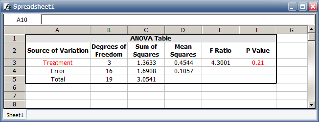
Then click the Detailed Summary link on the Main page of the control panel to view the ANOVA table of the results, as shown next.

From the ANOVA table, you can see that the p value is less than the risk level of 0.1 that was specified on the Analysis Settings page of the control panel, which is why the value is shown in red. This indicates that there is significant difference between the four operators.

Recreate P Value Using Function Wizard

To see how the p value is calculated, do the following:

Add a spreadsheet to the project by choosing Insert > Reports and Plots > Add Spreadsheet.

Return to the one-way ANOVA results and select the entire ANOVA table. Copy the table and paste it into the spreadsheet so it appears as shown next.

Select the populated cell in the F Ratio column (E3).
To use a name for this cell, choose Sheet > Format and View > More Settings > Define Name.

In the Name column, type "FRatio" then click the Active Cell(s) button to auto-set the definition to the cell currently selected in the Spreadsheet. Click Close to accept the definition and return to the spreadsheet.
Delete the value in the cell containing the p value (F3).
With cell F3 still selected, open the Function Wizard by choosing Sheet > Sheet Actions > Function Wizard.

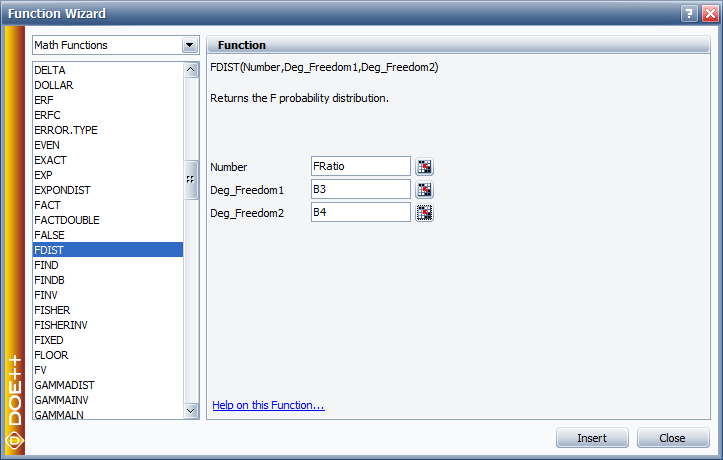
In the Function Wizard, scroll down the list of functions on the left and select FDIST. You can click the Help on this Function link in the Function area if you want to learn more about this function.

In the Number field, type "FRatio" to use the variable name you have defined as input. In the spreadsheet, select the cell that contains the degrees of freedom for Treatment (B3). Then return to the Function Wizard and click the Insert Workbook Reference icon next to the Deg_Freedom1 field. Use the same procedure to insert the degrees of freedom for Error in the Deg_Freedom2 field. The window will appear as shown next.

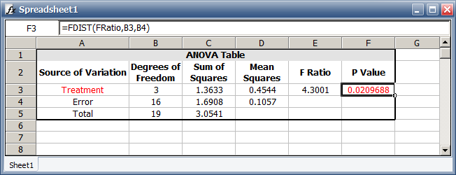
Click the Insert button to insert the function in the P Value cell that was selected when you opened the window. The spreadsheet will look like the one shown next.

When the P Value cell is selected, the Data Entry Box at the top of the window will display the formula that is being used to generate the value.